40 excel chart legend labels
Best Types of Charts in Excel for Data Analysis ... - Optimize Smart To add a chart to an Excel spreadsheet, follow the steps below: Step-1: Open MS Excel and navigate to the spreadsheet, which contains the data table you want to use for creating a chart. Step-2: Select data for the chart: Step-3: Click on the 'Insert' tab: Step-4: Click on the 'Recommended Charts' button: How to: Show or Hide the Chart Legend - DevExpress For example, to hide a legend entry, add a LegendEntry instance to the collection with the index set to the index of the selected entry. Next, set the LegendEntry.Hidden property to true. You can also change the font attributes of an individual entry by utilizing the LegendEntry.Font property. The example below demonstrates how to remove the ...
How to print a Gantt Chart view without table information - Office For Tables, click Task. Click the New button. In the Name box, enter No Table Info. In the first row, under Field Name, enter ID, and in the first row under Width, enter a zero (0). Click to select Show In Menu. Click OK, and then click Close. You can now use this table to print or preview a Gantt Chart view without table information as follows:

Excel chart legend labels
How to Switch Axes on a Scatter Chart in Excel - Appuals.com To try and switch the axes of a scatter chart using this method, you need to: Click anywhere on the scatter chart you watch to switch the axes to select it. You should now see three new tabs in Excel - Design , Layout, and Format. Navigate to the Design tab. In the Data section, locate and click on the Switch Row/Column button to have Excel ... Display more digits in trendline equation coefficients - Office Open the worksheet that contains the chart. Right-click the trendline equation or the R-squared text, and then click Format Trendline Label. Click Number. In the Category list, click Number, and then change the Decimal places setting to 30 or less. Click Close. Method 2: Microsoft Office Excel 2003 and earlier versions of Excel How to Test Graphs and Charts (Sample Test Cases) 19) Scroll-bar need to be available to see the entire graph. 20) Export the Graph in Excel or PDF and see how it looks. 21) Test the Graph report in all supported browsers. 22) Must use Standard Font Size and Font Style at Graph Dashboard. 23) Graph or chart name should be meaningful.
Excel chart legend labels. How to: Change the Display of Chart Axes - DevExpress How to: Change the Display of Chart Axes. Apr 27, 2022; 11 minutes to read; When you create a chart, its primary axes are generated automatically depending on the chart type.Most charts have two primary axes: the category axis (X-axis), usually running horizontally at the bottom of the plot area, and the value axis (Y-axis), usually running vertically on the left side of the plot area. 3-D ... Excel Pivot Table DrillDown Show Details To see the customer details for any number in the pivot table, use the Show Details feature. To see the underlying records for a number in the pivot table: In the Pivot Table, right-click the number for which you want the customer details. In the pop-up menu, click Show Details. TIP: Instead of using the Show Details command, you can double ... Chart js with Angular 12,11 ng2-charts Tutorial with Line, Bar, Pie ... datasets ({data: SingleDataSet, label: string}[]) - data see about, the label for the dataset which appears in the legend and tooltips; labels (Label[]) - x-axis labels. It's necessary for charts: line, bar and radar. And just labels (on hover) for charts: polarArea, pie, and a doughnut. How to: Display and Format Data Labels - DevExpress Add Data Labels to the Chart; Specify the Position of Data Labels; Apply Number Format to Data Labels; Create a Custom Label Entry; Add Data Labels to the Chart. Basic settings that specify the contents, position and appearance of data labels in the chart are defined by the DataLabelOptions object, accessed by the ChartView.DataLabels property ...
CD: Tornado Charts - Part 3 < Article < Blog - SumProduct Welcome back to our Charts and Dashboards blog series. This week, we'll finalise the formatting of our Tornado chart. ... We also want to edit the 'Legend Entries (Series)' to ensure that 'Series 1' has a more sensible name. Here, I'll choose the column header of 'High'. ... In later versions of Excel, take a detailed look at ... How to: Create and Modify a Chart - DevExpress Add or Remove Data Series. If you did not specify the range containing chart data in the ChartCollection.Add method, you can define it later by using one of the following approaches.. Pass the required data range to the ChartObject.SelectData method. The method's direction parameter allows you to specify the data direction: whether the series values are arranged in columns ... What would be a situation in which you could use an Excel chart to ... Weegy: What percentage of customer 101 buys product A, [ and what percentage of the same customer buys product B? -is a situation where you could use an Excel chart to present your data. ] Score .9771 User: What is entered into a cell that is typically numeric and can be used for calculations A. Value B. Tab C. Label D. Function How to: Display and Format Data Labels - DevExpress When data changes, information in the data labels is updated automatically. If required, you can also display custom information in a label. Select the action you wish to perform. Add Data Labels to the Chart. Specify the Position of Data Labels. Apply Number Format to Data Labels. Create a Custom Label Entry.
Tableau Essentials: Chart Types - The Text Table - InterWorks Since there are so many cool features to cover in Tableau, the series will include several different posts. The text table (also known as a crosstab) is essentially the same view you would see from an Excel data source or by clicking the View Data button in the Sidebar. The mark type is text, and the data is organized simply into rows and columns. Excel Tips & Solutions Since 1998 - MrExcel Publishing Strategy: An old Lotus 1-2-3 function—the N function—is still available in Excel. It turns out that N of a number is the number and N of any text is zero. Thus, you can add several N functions to a formula without changing the result, provided that they contain text. Excel add-in tutorial - Office Add-ins | Microsoft Docs command line. npm run start:web. To use your add-in, open a document in Excel on the web and then sideload your add-in by following the instructions in Sideload Office Add-ins in Office on the web. On the Home tab in Excel, choose the Toggle Worksheet Protection button. How to Change the Y Axis in Excel - Alphr In your chart, click the "Y axis" that you want to change. It will show a border to represent that it is highlighted/selected. Click on the "Format" tab, then choose "Format Selection ...
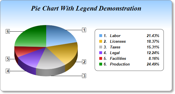
Pie Chart with Legend (2)
Free DMC Thread Inventory Spreadsheet | Lord Libidan A full excel spreadsheet tracker for DMC 6 strand threads! Includes all 500 "standard" threads, including new threads. Also now includes metallics, variations, Coloris, Etoile, and discontinued threads! ... - Thread conversion chart across 9 main thread brands One sheet is ordered by number, and another is by the official DMC color group. ...
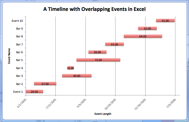
Excel Timelines
A Step-By-Step Guide on How to Make a Pie Chart in Excel 3. Select your data values and create the chart. Highlight the data range by clicking on the cell on the top left corner and dragging it until you've selected all the cells with values you wish to include in the pie chart. Then go to the top left corner of your window and click the "Insert" tab next to the "Home" tab.
![How to Make a Chart or Graph in Excel [With Video Tutorial] | Laptop Hustle](https://cdn2.hubspot.net/hub/53/hubfs/graph-label-size-excel.png?t=1529782838701&width=690&name=graph-label-size-excel.png)
How to Make a Chart or Graph in Excel [With Video Tutorial] | Laptop Hustle
Microsoft Excel - Wikipedia It introduced the now-removed Natural Language labels. This version of Excel includes a flight simulator as an Easter Egg. Excel 2000 (v9.0) ... Keyboard access for Pivot Tables and Slicers in Excel; New Chart Types; Quick data linking in Visio; ... Legend: Old version, not maintained Older version, still maintained
![How To Make A Two-Sided Bar Chart [VIDEO] - Annielytics.com](https://www.annielytics.com/wp-content/uploads/2012/12/sexy-bar-chart.png)
How To Make A Two-Sided Bar Chart [VIDEO] - Annielytics.com
Use defined names to automatically update a chart range - Office On the Insert tab, click a chart, and then click a chart type. Click the Design tab, click the Select Data in the Data group. Under Legend Entries (Series), click Edit. In the Series values box, type =Sheet1!Sales, and then click OK. Under Horizontal (Category) Axis Labels, click Edit. In the Axis label range box, type =Sheet1!Date, and then ...

33 Excel Legend Label - Labels Information List
12 Best Line Graph Maker Tools For Creating Stunning Line Graphs [2022 ... Plotly Chart Studio provides the solution for creating the graphs online. The graph can be created by importing the data from Excel, CSV, and SQL. It helps in creating many types of graphs and charts like bar charts, box plots, line graphs, dot plots, scatter plots etc.

30 How To Label Legend In Excel - Label Design Ideas 2020
How to Create Charts in Excel: Types & Step by Step Examples Below are the steps to create chart in MS Excel: Open Excel. Enter the data from the sample data table above. Your workbook should now look as follows. To get the desired chart you have to follow the following steps. Select the data you want to represent in graph. Click on INSERT tab from the ribbon. Click on the Column chart drop down button.
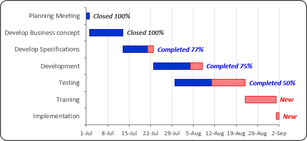
Gantt chart with progress
Chart control - Visual Studio (Windows) | Microsoft Docs The Chart control is a chart object that exposes events. When you add a chart to a worksheet, Visual Studio creates a Chart object that you can program against directly without having to traverse the Microsoft Office Excel object model. Applies to: The information in this topic applies to document-level projects and VSTO Add-in projects for Excel.
![How to Make a Chart or Graph in Excel [With Video Tutorial] | Charles A. Kush III](https://www.charleskush.com/wp-content/uploads/2018/06/format-legend-in-excel.png)
How to Make a Chart or Graph in Excel [With Video Tutorial] | Charles A. Kush III
PivotTable Aggregating Incorrect Data (Microsoft Excel) This can be especially true if you have deleted data, columns, or rows in the source data. To fix this potential issue, follow these general steps: Right-click a cell within the problem PivotTable. Excel displays a list of options. Choose PivotTable Options. Excel displays the PivotTable Options dialog box. Make sure the Data tab is displayed.
How to Create a Scatter Plot in Excel - TurboFuture - Technology
Compute and Display Heikin Ashi Charts in SQL Server and Excel Next, perform the selections to add the candlestick chart to the Excel tab. Start by selecting all the data for the chart. Next, choose Insert > Recommended Charts > All Charts > Stock. Then, select the candlestick chart image (see the image below). Close the Stock chart menu by clicking OK.
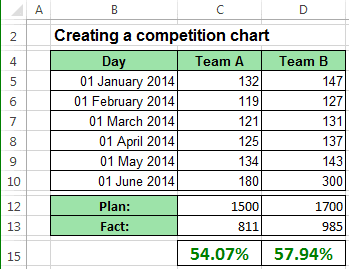
Creating a chart with dynamic labels - Microsoft Excel 2013
Excel table styles and formatting: how to apply, change and remove On the Design tab, in the Table Styles group, click the More button. Underneath the table style templates, click Clear. Tip. To remove a table but keep data and formatting, go to the Design tab Tools group, and click Convert to Range. Or, right-click anywhere within the table, and select Table > Convert to Range.

How To Label Legend In Excel Pie Chart - Chart Walls
How to Test Graphs and Charts (Sample Test Cases) 19) Scroll-bar need to be available to see the entire graph. 20) Export the Graph in Excel or PDF and see how it looks. 21) Test the Graph report in all supported browsers. 22) Must use Standard Font Size and Font Style at Graph Dashboard. 23) Graph or chart name should be meaningful.
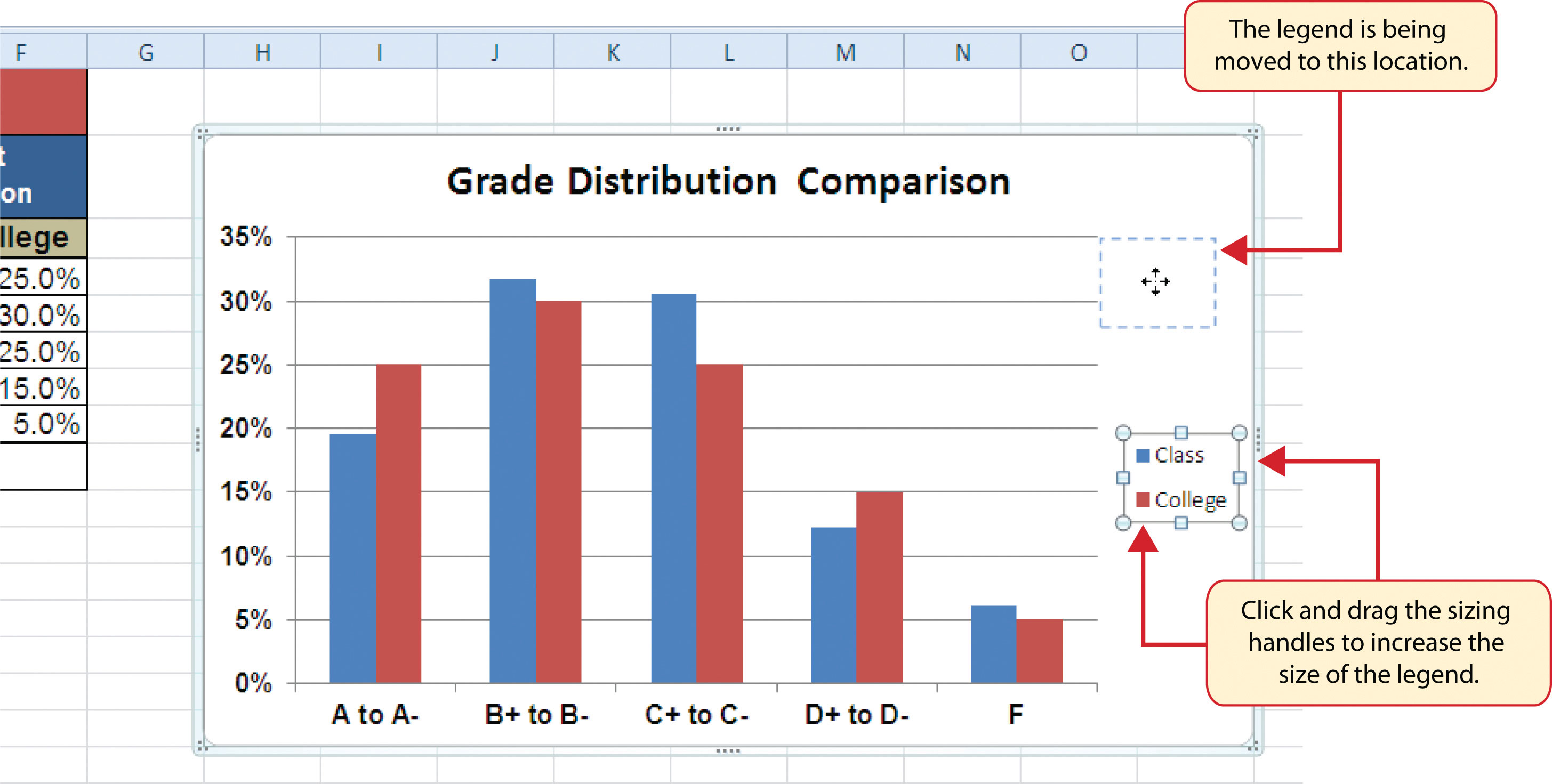
Presenting Data with Charts
Display more digits in trendline equation coefficients - Office Open the worksheet that contains the chart. Right-click the trendline equation or the R-squared text, and then click Format Trendline Label. Click Number. In the Category list, click Number, and then change the Decimal places setting to 30 or less. Click Close. Method 2: Microsoft Office Excel 2003 and earlier versions of Excel

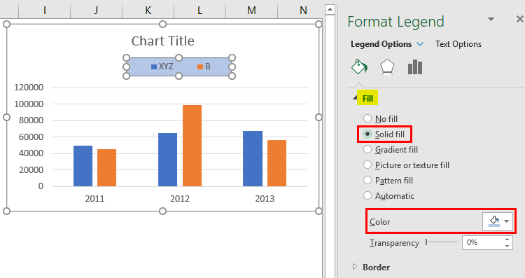
Excel Charts with Dynamic Title and Legend Labels | ExcelDemy
How to Switch Axes on a Scatter Chart in Excel - Appuals.com To try and switch the axes of a scatter chart using this method, you need to: Click anywhere on the scatter chart you watch to switch the axes to select it. You should now see three new tabs in Excel - Design , Layout, and Format. Navigate to the Design tab. In the Data section, locate and click on the Switch Row/Column button to have Excel ...
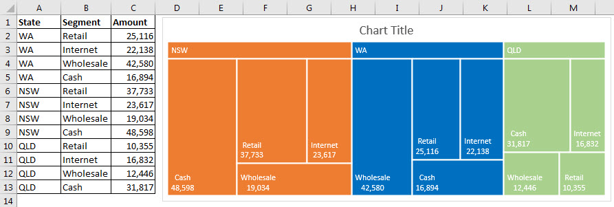
TreeMap a new chart in Excel 2016 | A4 Accounting

Five tips for enhancing Excel charts - TechRepublic
30 How To Label Legend In Excel - Label Design Ideas 2020

How to Create a Scatter Plot in Excel | TurboFuture
Chart axes, legend, data labels, trendline in Excel - Tech Funda
Post a Comment for "40 excel chart legend labels"