44 multiple data labels excel pie chart
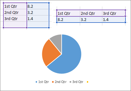
Add or remove data labels in a chart - support.microsoft.com Click the data series or chart. To label one data point, after clicking the series, click that data point. In the upper right corner, next to the chart, click Add Chart Element > Data Labels. To change the location, click the arrow, and choose an option. If you want to show your data label inside a text bubble shape, click Data Callout. How to Combine or Group Pie Charts in Microsoft Excel Click on the first chart and then hold the Ctrl key as you click on each of the other charts to select them all. Click Format > Group > Group. All pie charts are now combined as one figure. They will move and resize as one image. Choose Different Charts to View your Data
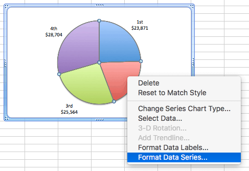
Creating Pie Chart and Adding/Formatting Data Labels (Excel) Creating Pie Chart and Adding/Formatting Data Labels (Excel)

Multiple data labels excel pie chart
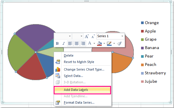
Pie Charts in Excel - How to Make with Step by Step Examples Task b: Add data labels and data callouts. Step 3: Right-click the pie chart and expand the "add data labels" option. Next, choose "add data labels" again, as shown in the following image. Step 4: The data labels are added to the chart, as shown in the following image. How to add data labels from different column in an Excel chart? This method will introduce a solution to add all data labels from a different column in an Excel chart at the same time. Please do as follows: 1. Right click the data series in the chart, and select Add Data Labels > Add Data Labels from the context menu to add data labels. 2. How to Show Percentage and Value in Excel Pie Chart - ExcelDemy Table of Contents hide. Download Practice Workbook. Step by Step Procedures to Show Percentage and Value in Excel Pie Chart. Step 1: Selecting Data Set. Step 2: Using Charts Group. Step 3: Creating Pie Chart. Step 4: Applying Format Data Labels. Conclusion. Related Articles.
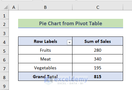
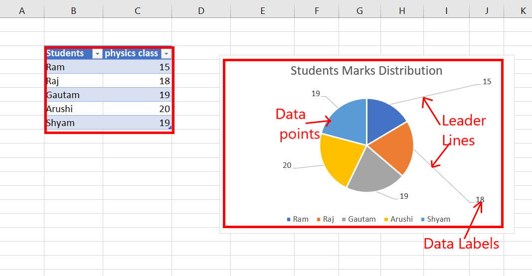
Multiple data labels excel pie chart. How to group (two-level) axis labels in a chart in Excel? - ExtendOffice You can do as follows: 1. Create a Pivot Chart with selecting the source data, and: (1) In Excel 2007 and 2010, clicking the PivotTable > PivotChart in the Tables group on the Insert Tab; (2) In Excel 2013, clicking the Pivot Chart > Pivot Chart in the Charts group on the Insert tab. 2. In the opening dialog box, check the Existing worksheet ... How to display leader lines in pie chart in Excel? - ExtendOffice To display leader lines in pie chart, you just need to check an option then drag the labels out. 1. Click at the chart, and right click to select Format Data Labels from context menu. 2. In the popping Format Data Labels dialog/pane, check Show Leader Lines in the Label Options section. See screenshot: Excel Pie Chart - How to Create & Customize? (Top 5 Types) Step 1: Click on the Pie Chart > click the ' + ' icon > check/tick the " Data Labels " checkbox in the " Chart Element " box > select the " Data Labels " right arrow > select the " More Options… ", as shown below. The " Format Data Labels" pane opens. How to add or move data labels in Excel chart? - ExtendOffice In Excel 2013 or 2016. 1. Click the chart to show the Chart Elements button . 2. Then click the Chart Elements, and check Data Labels, then you can click the arrow to choose an option about the data labels in the sub menu. See screenshot: In Excel 2010 or 2007. 1. click on the chart to show the Layout tab in the Chart Tools group. See ...
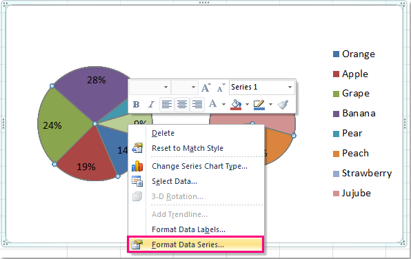
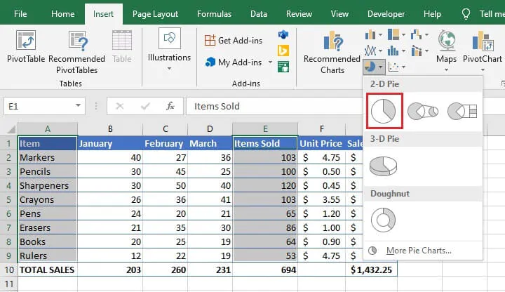
Create a multi-level category chart in Excel - ExtendOffice Create a multi-level category chart in Excel A multi-level category chart can display both the main category and subcategory labels at the same time. When you have values for items that belong to different categories and want to distinguish the values between categories visually, this chart can do you a favor. How to Make a Pie Chart in Excel & Add Rich Data Labels to The Chart! Creating and formatting the Pie Chart 1) Select the data. 2) Go to Insert> Charts> click on the drop-down arrow next to Pie Chart and under 2-D Pie, select the Pie Chart, shown below. 3) Chang the chart title to Breakdown of Errors Made During the Match, by clicking on it and typing the new title. How to Make a Pie Chart with Multiple Data in Excel (2 Ways) - ExcelDemy First, to add Data Labels, click on the Plus sign as marked in the following picture. After that, check the box of Data Labels. At this stage, you will be able to see that all of your data has labels now. Next, right-click on any of the labels and select Format Data Labels. After that, a new dialogue box named Format Data Labels will pop up. updating data labels in pie charts, - Microsoft Community The data labels in my pie chart won't update. My data labels use & to combine data from three cells into a label and the result is the data label. ... Excel; Microsoft 365 and Office; Search Community member; JE. John E-154 Created on September 21, 2022.
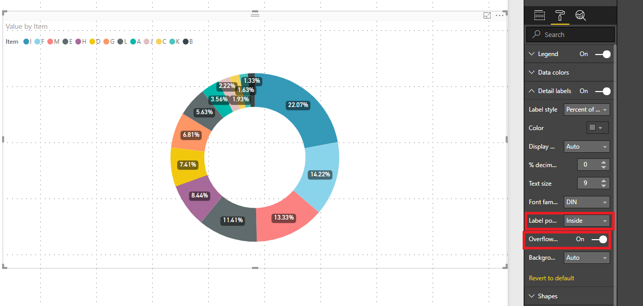
How to Create and Format a Pie Chart in Excel - Lifewire Select the plot area of the pie chart. Right-click the chart. Select Add Data Labels . Select Add Data Labels. In this example, the sales for each cookie is added to the slices of the pie chart. Change Colors When a chart is created in Excel, or whenever an existing chart is selected, two additional tabs are added to the ribbon. Show multiple data lables on a chart - Power BI For example, I'd like to include both the total and the percent on pie chart. Or instead of having a separate legend include the series name along with the % in a pie chart. I know they can be viewed as tool tips, but this is not sufficient for my needs. Many of my charts are copied to presentations and this added data is necessary for the end ... Excel Pie Chart Labels on Slices: Add, Show & Modify Factors - ExcelDemy It will help us to separate the data labels from the pie chart. 📌 Steps: First of all, click on the data labels on the pie chart. Now, in the Format tab, click on the drop-down arrow of the Shape Outline from the Shapes Style group. Then, choose your desired color for the shape outline. We choose White, Background 1 color for our shape outline. Formatting data labels and printing pie charts on Excel for Mac 2019 ... Here's a work around I found for printing pie charts. Still can't find a solution for formatting the data labels. 1. When printing a pie chart from Excel for mac 2019, MS instructions are to select the chart only, on the worksheet > file > print. Excel is supposed to print the chart only (not the data ) and automatically fit it onto one page.
How to Show Percentage in Pie Chart in Excel? - GeeksforGeeks
Pie Chart in Excel - Inserting, Formatting, Filters, Data Labels Click on the Instagram slice of the pie chart to select the instagram. Go to format tab. (optional step) In the Current Selection group, choose data series "hours". This will select all the slices of pie chart. Click on Format Selection Button. As a result, the Format Data Point pane opens.
Solved: How to show all detailed data labels of pie chart ...
Everything You Need to Know About Pie Chart in Excel - SpreadsheetWeb How to Make a Pie Chart in Excel. Start with selecting your data in Excel. If you include data labels in your selection, Excel will automatically assign them to each column and generate the chart. Go to the INSERT tab in the Ribbon and click on the Pie Chart icon to see the pie chart types. Click on the desired chart to insert.

How to Make Pie Chart with Labels both Inside and Outside ...
Dynamic pie chart labels | MrExcel Message Board Messages. 8. Jun 18, 2020. #1. Hi. Wondering if you clever ppl can help me. I have created PivotChart I have used a pie chart to display two bits of data. I have created a slicer that filters the pivot chart (this is into years). The problem I am having is that the internal Data labels withing the pie chart that shoes the percentage, keeps ...
How to Create a Pie Chart in Excel | Smartsheet
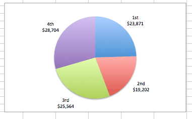
Multiple Data Labels on a Pie Chart | MrExcel Message Board So I have a table with 8 rows and 3 columns. This table includes: Column 1 - shipment name Column 2 - shipment cost Column 3 - shipment weight I have created a pie chart from this table, which covers the first two columns. Displayed next to each slice is a label with the shipment name, shipment cost, and percent share of the pie.

How to Create a Pie Chart in Excel - Displayr
Change the format of data labels in a chart To get there, after adding your data labels, select the data label to format, and then click Chart Elements > Data Labels > More Options. To go to the appropriate area, click one of the four icons ( Fill & Line, Effects, Size & Properties ( Layout & Properties in Outlook or Word), or Label Options) shown here.
How to create pie of pie or bar of pie chart in Excel?
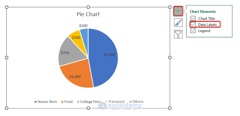
Create a Pie Chart in Excel (In Easy Steps) - Excel Easy Create the pie chart (repeat steps 2-3). 7. Click the legend at the bottom and press Delete. 8. Select the pie chart. 9. Click the + button on the right side of the chart and click the check box next to Data Labels. 10. Click the paintbrush icon on the right side of the chart and change the color scheme of the pie chart.

Add or remove data labels in a chart
Multiple data labels (in separate locations on chart) Re: Multiple data labels (in separate locations on chart) You can do it in a single chart. Create the chart so it has 2 columns of data. At first only the 1 column of data will be displayed. Move that series to the secondary axis. You can now apply different data labels to each series. Attached Files 819208.xlsx (13.8 KB, 265 views) Download

How to Change Excel Chart Data Labels to Custom Values?
How to Make Pie of Pie Chart in Excel (with Easy Steps) Step-04: Employing Data Labels Format You can also make changes to data labels. Which will make your information more visual. At first, you have to click on the + icon. Then, from the Data Labels arrow >> you need to select More Options. At this time, you will see the following situation.

Power BI Pie Chart - Complete Tutorial - SPGuides
Edit titles or data labels in a chart - support.microsoft.com To edit the contents of a title, click the chart or axis title that you want to change. To edit the contents of a data label, click two times on the data label that you want to change. The first click selects the data labels for the whole data series, and the second click selects the individual data label. Click again to place the title or data ...
How to Make a Pie Chart with Multiple Data in Excel (2 Ways)
Move data labels - support.microsoft.com Right-click the selection > Chart Elements > Data Labels arrow, and select the placement option you want. Different options are available for different chart types. For example, you can place data labels outside of the data points in a pie chart but not in a column chart.
How to fix wrapped data labels in a pie chart | Sage Intelligence
How to Show Percentage and Value in Excel Pie Chart - ExcelDemy Table of Contents hide. Download Practice Workbook. Step by Step Procedures to Show Percentage and Value in Excel Pie Chart. Step 1: Selecting Data Set. Step 2: Using Charts Group. Step 3: Creating Pie Chart. Step 4: Applying Format Data Labels. Conclusion. Related Articles.

How to Create a Pie Chart in Excel | Smartsheet
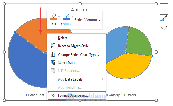
How to add data labels from different column in an Excel chart? This method will introduce a solution to add all data labels from a different column in an Excel chart at the same time. Please do as follows: 1. Right click the data series in the chart, and select Add Data Labels > Add Data Labels from the context menu to add data labels. 2.
/Capture-e92aa05671d543ceaf94080eb2687619.JPG)
Understanding Excel Chart Data Series, Data Points, and Data ...
Pie Charts in Excel - How to Make with Step by Step Examples Task b: Add data labels and data callouts. Step 3: Right-click the pie chart and expand the "add data labels" option. Next, choose "add data labels" again, as shown in the following image. Step 4: The data labels are added to the chart, as shown in the following image.

Microsoft Excel Tutorials: Add Data Labels to a Pie Chart

How to Show Percentage in Pie Chart in Excel? - GeeksforGeeks
5 New Charts to Visually Display Data in Excel 2019 - dummies

Add or remove data labels in a chart
How to Make a Pie Chart with Multiple Data in Excel (2 Ways)
Automatically Group Smaller Slices in Pie Charts to one big Slice
Select data for a chart
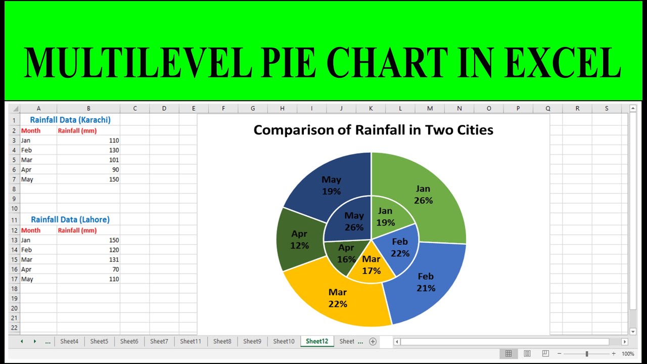
How to Make Multilevel Pie Chart in Excel

How to create pie of pie or bar of pie chart in Excel?
How to create pie of pie or bar of pie chart in Excel?

Creating Graphs in Excel 2013
Create a Pie Chart in Excel (In Easy Steps)
How to Make a Pie Chart with Multiple Data in Excel (2 Ways)

How to make a pie chart in Excel

Add or remove data labels in a chart

Everything You Need to Know About Pie Chart in Excel

How to make a Pie Chart in Excel

How to Create a Pie Chart in Excel | Smartsheet

Excel charts: add title, customize chart axis, legend and ...
How to Add Leader Lines in Excel? - GeeksforGeeks
How to Make a Pie Chart with Multiple Data in Excel (2 Ways)
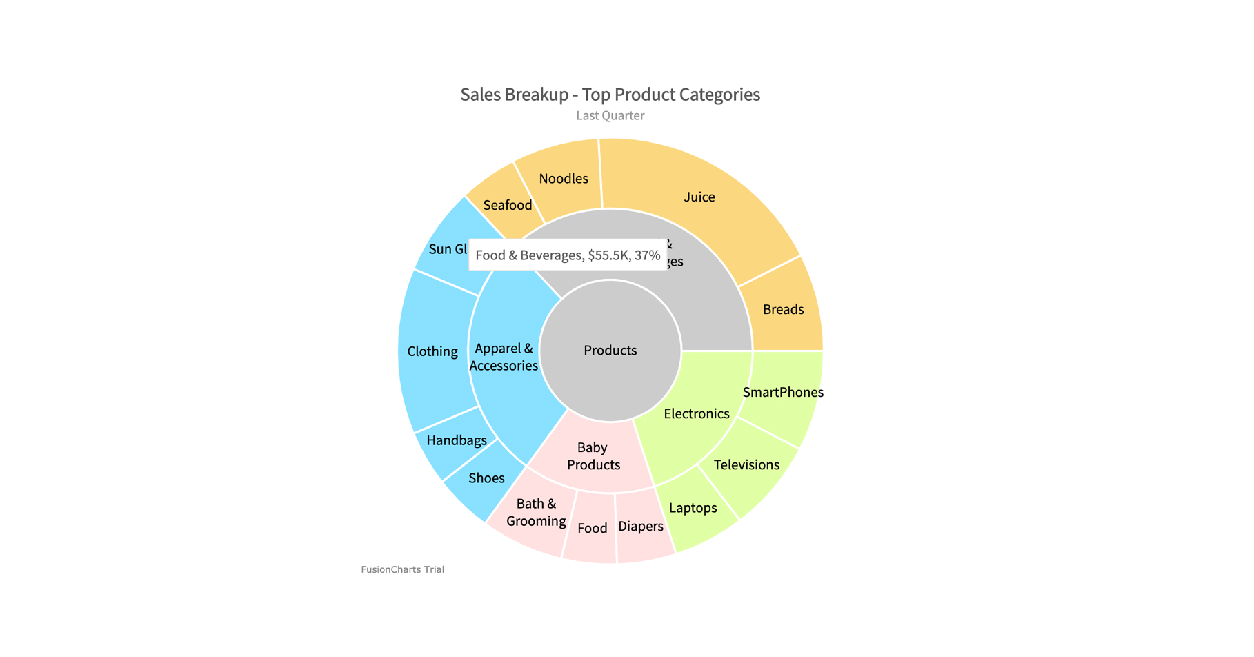
Multi-level Pie Chart | FusionCharts

Power BI Pie Chart - Complete Tutorial - EnjoySharePoint
How to Create a Pie Chart in Excel | Smartsheet

How to Data Labels in a Pie chart in Excel 2010
How to Make a Pie Chart in Excel | GoSkills
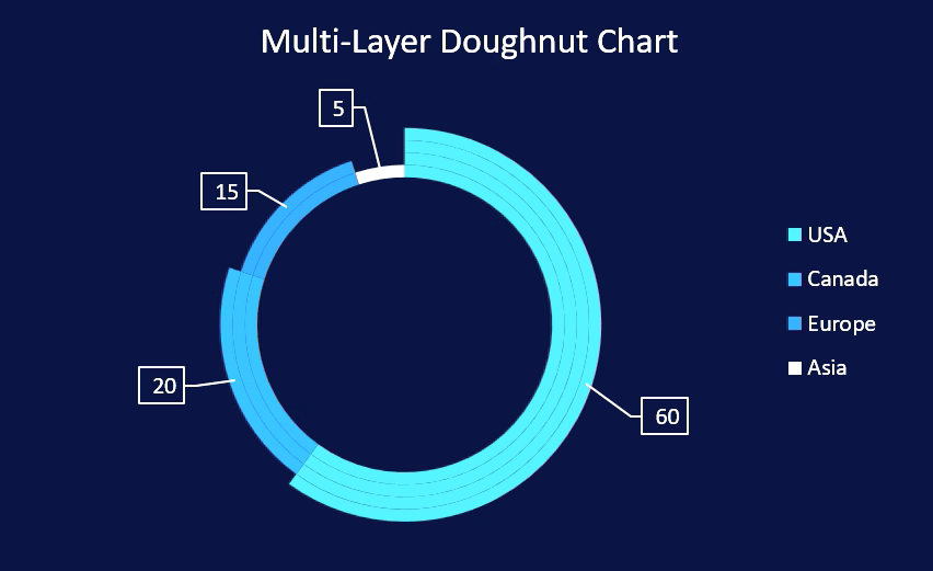
How to create a creative multi-layer Doughnut Chart in Excel
How to Make a Pie Chart with Multiple Data in Excel (2 Ways)

Improve your X Y Scatter Chart with custom data labels
Move and Align Chart Titles, Labels, Legends with the Arrow ...

Add or remove data labels in a chart
Post a Comment for "44 multiple data labels excel pie chart"